Run a simple kinetic Monte Carlo simulation for catalytic reaction kinetics in Python
Introduction:
Kinetic Monte Carlo (kMC) is a powerful tool for studying reaction kinetics when the set of important steps becomes too complicated for exact analysis of deterministic rate equations. kMC is used to generate stochastic trajectories through the space of possible metastable states that the system can adopt. Important information about reaction dynamics can be extracted from these trajectories, such as reaction rates and rate constants. As a first step to running kMC simulations, a simple kMC code is developed to simulate a catalytic reaction as it proceeds towards thermodynamic equilibrium. The equilibrium behavior is shown to be consistent with that determined from the kinetic parameters. The next parts in the series will show how reaction rates are obtained from these simulations.
Tutorial:
(link to code: https://github.com/ari-fischer/kinetics_tutorial/tree/9e7ea49ca8f6c48bcc8ef1c22e1c0fb8d78b9a61/KMC_tutorials)
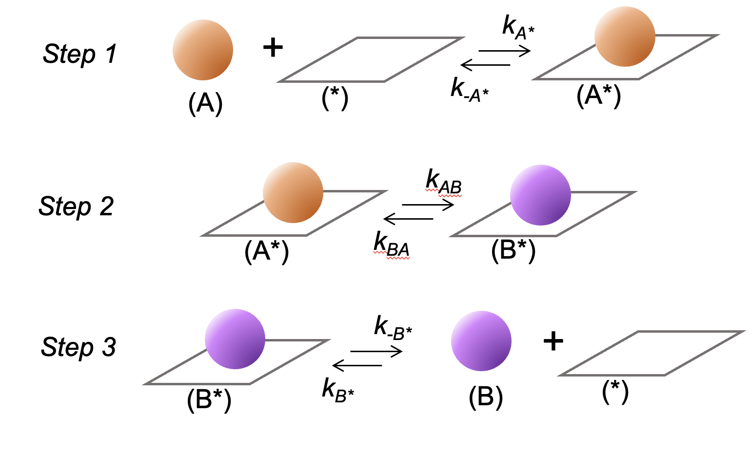
A simple catalytic reaction network for the conversion of species A to B is depicted in Scheme 1. It consists of A adsorption at a catalytic site (denoted by *) to form A* (step 1), A* conversion to B* (step 2), and B* desorption to form B. Acid-catalyzed 1-butene isomerization to 2-butene (Scheme 2) is one example of a reaction that follows these steps.
Scheme 1: A sequence of elementary steps for the conversion of species A to B on a catalytic site (denoted by *). The ki terms represent forward and reverse rate constants for each reaction step.

Scheme 2: A sequence of elementary steps for acid-catalyzed 1-butene isomerization to 2-butene.

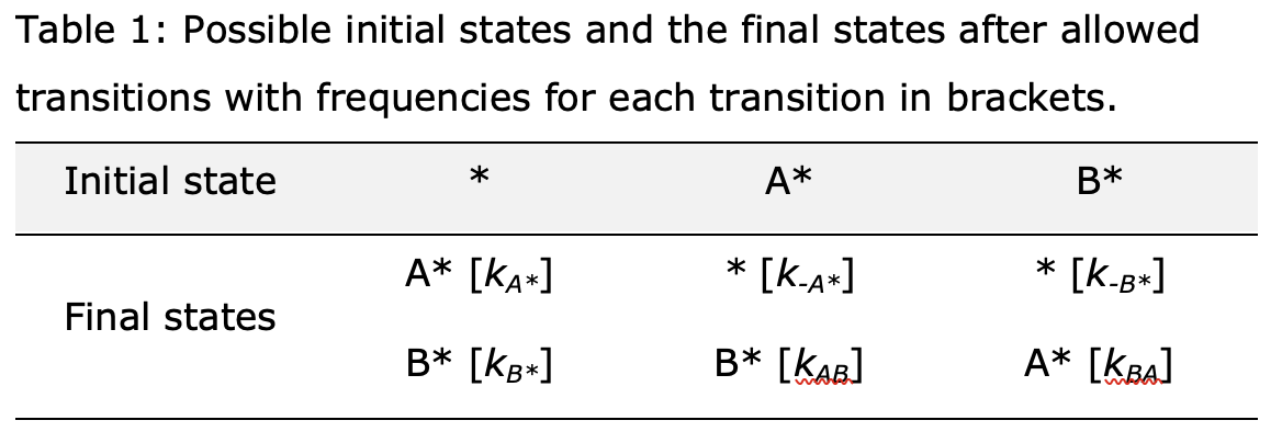
Scheme 1 considers a catalytic site (*) that can be either (i) empty, (ii) A-covered, or (iii) B-covered. Each state can transition into others with frequencies represented by the rate constant for the elementary reactions (Scheme 1). Table 1 shows the set of possible initial states and the final states that are formed after a transition along with the frequencies of these transitions.

The procedure required to execute a transition from a given initial state is shown next as an illustrative example. The reader is referred to publications by Peters [1] and Andersen et al. [2] for more details regarding the algorithm and its implementation. The procedure for transition from an initial state, i, is outlined in the following:
-
Identify all possible transitions from initial i state and their corresponding frequencies.
-
Compute the net rate of transition from state i (denoted by ki,tot) from the sum over the frequencies of each possible transition to the new state j (ki,tot = ∑j ki,j).
-
Select a random number (u1) between 0 and 1.
-
Find the value of j that satisfies the following relation to determine which transition occurs:
ki,j-1 / ki,tot < u1 < ki,j / ki,tot
-
Replace state i with the selected state j.
-
Select another random number (u2) between 0 and 1.
-
Update the simulation time (t) by adding the waiting time (Δt) computed by sampling the probability density for the first transition out of state I to occur (Δt =-ln(u2)/ki,tot) [1].
-
Repeat steps 1-8.
The steps outlined above are implemented in a Jupyter notebook (with Python 3) to simulate the reaction dynamics. A sample code is available on Github (see appendix for details).
First, numpy, scipy, and pyplot modules are imported:
import numpy as np
import scipy as sci
import matplotlib.pyplot as plt
Next, the values of the rate constants in Scheme 1 are specified (Table 2).

kA_a0 = 10 # A adsorption constant
kB_a0 = 1 # B adsorption constant
kA_d = 1 # A desorption constant
k_AB = .1 # A conversion to B
kB_d = .1 # B desorption constant
k_BA = .01 # B conversion to A
The state of the system is then initialized. At time zero, the surface is uncovered. This is denoted by an index of 0. Indexes of 1 and 2 represent A- and B-covered surfaces, respectively. The active site is exposed to a bath initially containing 1000 molecules of A and zero molecules of B. The simulation with proceed for 100000 events:
# initial parameters #
t = 0 # initial time
L = 0 # initial state: 0 – empty; 1 – A*; 2 – B*
N_A = 1000 # number of A
N_B = 0 # number of B
trials = 100000
# vector for A, B, and t #
N_As = list([N_A])
N_Bs = list([N_B])
ts = list([t])
The trajectory is now ready to be simulated with the parameterized rate constants and initial state specified. The specified number of trials are executed by implementation in a for loop. Each execution of the loop performs steps 1-7, then repeats the same code using the final state from the previous execution. The following code uses an intuitive (albeit inefficient) implementation with nested if statements used for purposes of illustration. To start, the loop is entered and two random numbers are drawn:
for i in range(trials):
u1 = np.random.rand(1) #rand for the particular process selected
u2 = np.random.rand(1) #rand for the time step
Next, an if statement is used to determine which process to execute depending on the initial state:
if L == 0: #vacant site
…
elif L == 1: # A covered
…
elif L == 2: #B covered
…
Then, the rate constants for transition from the current state are determined and constructed into an array (with an initial state of 0 as an example). The rate constant for A and B adsorption are multiplied by the molar fractions of A and B, respectively, to get rates:
if L == 0: #vacant site
#adsorption
kA_a = kA_a0 * (N_A)/(N_A + N_B) #adsorption rate of A based on prevalent A mole fraction
kB_a = kB_a0 * (N_B)/(N_A + N_B) #adsorption rate of B based on prevalent B mole fraction
ks = np.array([kA_a,kB_a])
Then, the move to take is selected by comparing u~1~ to a cumulative array of the ks of possible events.
k_tot = np.sum(ks) # get the total rate of transition from the sum of ks
k_stack = np.cumsum(ks) # get a cumulative array of ks for event selection
select = n1*k_tot # find the value in the cumulative array to select
#pick the first one that is larger than the select criteria
indexes = np.arange(len(k_stack))
ind_move = indexes[k_stack>select][0]
Next, the state of the system is updated depending on the move selected. If the move is 0, meaning A adsorbs, the next state becomes 1 (A*) and one A molecule is removed from the gas phase.
if ind_move == 0:
L = 1
N_A += -1
elif ind_move == 1:
L = 2
N_B += -1
The rate constants for transition from the initial state are obtained and the next move is executed using a similar procedure to that outlined above when L= 1 or 2. The waiting time is then evaluated outside of the if statement using the frequency for transition computed and updates the simulation time:
t += - np.log(n2)/k_tot #t estable
Finally, the new times and numbers of A and B are appended to their respective vectors to tract their time evolutions:
ts.append(t[0])
N_As.append(N_A)
N_Bs.append(N_B)…
The system is evolved using the code above for 100000 steps. The first few states for a single trajectory are printed with corresponding time intervals as follows:
Ls = (0,1,0,1,2,0,1,0,1, …)
ts = (0.26, 0.48, 0.15, 0.21, 0.05, 0.33, 1.7, …)
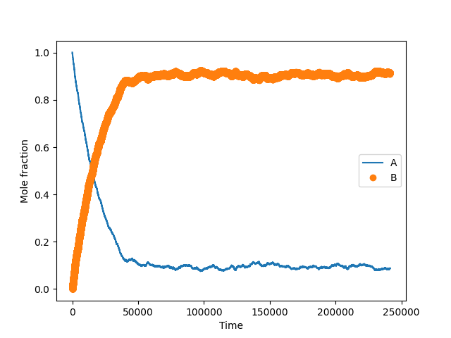
The mole fractions of A (yA) and B (yB) species present in the gas phase are plotted as a function of the simulation time (Figure 1). Recall that the number of A or B decreases by one unit every time the state transitions from 0 to 1 or 2, respectively. Their values increase by one unit every time the state transitions from either 1 or 2 to 0, respectively. The fraction of A decreases asymptotically towards an equilibrium value of around 0.11 while B increases asymptotically towards an equilibrium value of around 0.89. Their values approach this stable equilibrium value as fractions of A and B adjust to establish detailed balance.

The fraction of B (divided by A corresponds to an equilibrium constant (KAB) of 9.9 via through KAB = yB / yA. The equilibrium behavior is compared to the value obtained from deterministic equations derived from the elementary steps in Scheme 1. A relation between reactants and products for each elementary step in quasi-equilibrium is obtained as follows:

Here, the θ terms denote fractional surface coverages of A, B, or empty (*) sites. Solving this set of algebraic equations for the yB / yA ratio gives a definition of KAB in terms of the forward and reverse rate constants in Scheme 1:

The KAB determined from these rate constants is 10.0, in close agreement with the value obtained from the stable behavior in the trajectory.
Exercises:
-
How do changes to the rate constants affect the equilibrium ratio?
-
How do changes to the rate constants affect the time it takes to reach a stable A-B ratio?
-
How can the code be modified to obtain steady-state reaction rates for A conversion to B at a fixed A mole fraction (yA)?
The next post in the series will show a solution to exercise 3
References:
[1] Reaction rate theory and rare events. B Peters. Elsevier, 2017. ISBN: 978-0-444-56349-1
[2] Andersen M, Panosetti C, Reuter K. A Practical Guide to Surface Kinetic Monte Carlo Simulations. Front Chem. 2019;7:202.
Appendix:
The sample code is available as a Jupyter notebook entitled “kMC_A_B_rxn_single_site_eq.ipynb” at the ari-fischer GitHub page (https://github.com/ari-fischer/) in the “kinetics_tutorial” repository under the “KMC_tutorials” folder