Steady-state kinetics with kinetic Monte Carlo in Python and the connection to mean field kinetic descriptions.

Introduction:

The previous guide (https://ari-fischer.github.io/site/kinetics/tutorials/2023/07/23/KMC_tutorial_1_equilibrium.html) introduced the concept of kinetic Monte Carlo (kMC) and built a code to simulate the dynamics of reactant A conversion into product B at a catalytic surface. The mole fraction of A and B that the catalyst surface was exposed to was evolved from an initial state consisting of only A to a final state reflecting thermodynamic equilibrium between A and B. The true power of kMC, however, lies in determining kinetic behaviors for complex systems, rather than determining thermodynamic endpoints which are independent of the path taken by the system. The reader is referred to Andersen et al. for some examples where kMC has been applied to study the kinetics of surface diffusion, crystal growth, and heterogeneous catalysis [1].

Here, a kMC model of the same A to B reaction is employed to simulate steady-state dynamics and obtain reaction rates and effective rate constants. These rates and parameters are shown to be identical to those obtained by analyzing Langmuir-Hinshelwood kinetics for the same reaction. In doing so, it becomes clear how dynamic behaviors gleaned from kMC simulations reflect the same kinetics as those from mean-field descriptions of reaction kinetics.

Analyzing steady-state kinetics with mean field kinetic descriptions:

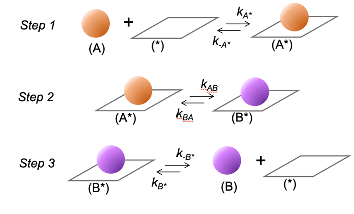
Scheme 1 shows the sequence of elementary steps that mediates A conversion to B on a catalyst surface. Step 1 shows the adsorption of A to a vacant *-site (denoted by *) to form A to form A*. Step 2 shows the conversion of A* to B* at the surface. Step 3 shows the desorption of B* to form the product B and a vacant *-site.

Scheme 1: A sequence of elementary steps for the conversion of species A to B on a catalytic site (denoted by *). The k_i terms represent forward and reverse rate constants for each reaction step.

Mean field rate expressions for each of the elementary step in Scheme 1 occurring on L_* active sites are obtained by considering each step to be reversible and with their forward and reverse rates related to reactant mole fractions from the law of mass action (i.e. that the rate of reaction is proportional to the product of reactant thermodynamic activities) [2]:

Here, y_A and y_B are the mole fractions of A and B, respectively; θ_A, θ_B, and θ are the fractional surface coverages of *A, B and vacancies on L* sites; and ki are rate constants with corresponding steps denoted in Scheme 1.</sub>

An analytical expression for the rate of B formation can be derived based on the following assumptions consistent with the values of rate constants in Table 1. First, B* desorbs much faster than it reacts at the surface to re-form A* (k_-B/k_BA=100000), indicating that B* formation in Step 2 is irreversible. The rate of Step 2 can therefore be restated as:

Secondly, A* desorbs much faster than it reacts to form B* (k_-A/k_AB=100) indicating that Step 1 occurs at quasi-equilibrium (i.e. the forward and reverse rates of Step 1 are both much larger than the net rate of reaction). Approximating the net rate of Step 1 as zero gives the quasi-equilibrium coverage of A*:

The coverage of vacant *-sites, A*, and B* are related by the conservation of occupied and unoccupied L* sites, given by:

The coverage of B* is assumed to be negligible at low conversion (low y_B) because B* desorbs faster than it adsorbs (k_-B/k_B=10). An expression for θ_* can be obtained by neglecting the θ_B term, replacing θ_A with its value from equation 5, and solving for θ_*:

The net rate of B formation is obtained by replacing the θ_* term in equation 5 with its value from equation 7, and then substituting the resulting expression for θ_A into equation 4:

This equation thus relates the rate of B formation normalized by the number of *-sites to the mole fraction of A and the kinetic constants for its reaction at *-sites.

Figure 1 shows the effect of y_A on the coverages of vacant *-sites and A* (left) and on the rate of B formation (right) (with y_A changed by diluting A with an inert gas like He). Intuitively, coverages of A* increase and vacant * decrease as y_A increases and A adsorption becomes more favorable. The rate of B formation increases proportional to the A* coverage, reflecting the functional form of equation 4.

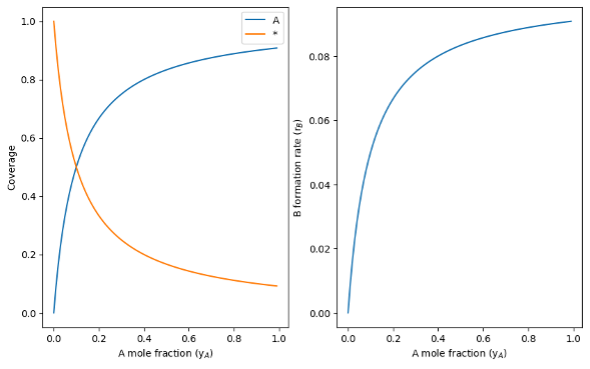
Figure 1: A* and vacant *-site coverages (left) and B formation rate (right) as a function of A mole fraction (y_A).

Equation 8 relates the macroscopic rate of B formation to the macroscopic mole fraction of reactant A. Its derivation requires a fractional coverage of active sites to be defined, which implicitly requires a large number of active sites so that fractional coverages behave as continuous functions. This rate expression is a faithful description of reactivity only at length and time scales in the thermodynamic limit where these macroscopic observables are significant. The single active site considered in the kMC model from the previous walkthrough, on the other hand, considers only a single active site, that is either occupied or unoccupied, but cannot partially occupied. Moreover, products are formed one at a time by the desorption of B from a B-covered *-site in a stochastic manner, rather than forming continuously at a constant rate.

The reaction we are considering has properties that enables its microscopic and macroscopic observables to be related. First, it is Markovian, meaning that the next step taken from the current state depends only on the present configuration, but not on the previous steps [2]. It is also ergodic, meaning that all possible states of the system are dynamically accessible from one another [2]. Finally, the process has time-translational symmetry, meaning that the probabilities for transitioning from one state to another depends only on relative, but not absolute, time [2]. For systems with these properties, the probability of finding the system in each of the possible states follows a unique distribution after a long enough simulation time.

In the example catalytic reaction, for instance, the average amount of time that the system is found in states A*, B*, or * reflects the unique probability of finding the system in that state for a simulation with a long enough time elapsed. This characteristic implies that simulating the behavior of a single site over a long enough simulation time gives time-averaged representations of macroscopic observables like coverages and B formation rates, which can be compared with those quantities obtained from the mean field kinetic models derived above. These time-averaged quantities are calculated next from a kMC simulation.

Adapting the kMC code to simulate steady-state behaviors:

(link to code: https://github.com/ari-fischer/kinetics_tutorial/tree/92e92c102a27a431a2ba9d655732d157fef8f4dc/KMC_tutorials)

The model developed in the previous guide (to simulate thermodynamic behaviors) includes a bath of reactant A and product B, initialized at zero time as follows:

#initialize:

N_A = 1000

N_B = 0

The catalyst surface interacts with the reservoir in each step of the kMC simulation by either (i) removing A or B from the reservoir if an adsorption event took place, or (ii) adding A or B to the reservoir if the desorption of A* or B*, respectively, took place. For instance, if the current state was a vacant site, and the selected move for that step was to adsorb A, then one A was removed from the reservoir (“N_A += -1”) and the state of the site was changed to the A-covered state (“L = 1”), implemented as follows:

for i in range(trials): #vacant site

…

if L == 0: #vacant site

…

if ind_move == 0: # A adsorption selected

L = 1 # change from vacant site to A-covered site (A*)

N_A += -1 # remove one species A from the reservoir

As the simulation progresses, A is progressively consumed and B generated until the ratio of A to B in the reservoir establishes thermodynamic equilibrium. Such equilibration occurs because the probabilities that A and B adsorb to a vacant site are proportional to their mole fractions in the reservoir. Consequently, as A is depleted, A* formation from A adsorption becomes slower, while an increase in B increases the rate of B* formation from B adsorption.

Steady-state kinetics for A conversion to B are instead obtained by fixing the mole fractions of A and B in the reservoir so that the probabilities for A and B adsorption do not change with the simulation time. This is achieved by simply commenting out the “N_A += -1” line from the previous simulation so that the A-adsorption step does not affect the amount of A in the reservoir. The same is done for the B-desorption step (“N_B += 1”). We still, however, want to keep track of the number of products formed during a simulation, so the we define a number of products formed “N_P” initialized as:

N_P = 0

…

N_Ps = list([N_P])

And we add 1 to this every time B desorbs from the site:

for i in range(trials): #vacant site

…

elif L == 2: #vacant site

…

if ind_move == 0: # A adsorption selected

L = 0

N_P += 1#add this one in as a tracer of products formed

This N_P is simply a tracker of the number of B products formed, but does not influence the frequencies of any steps (because no rate constants depend on a P mole fraction).

Figure 2 shows the number of B products formed (from N_Ps) as a function of simulation time for a simulation of 100,000 trial steps. The number of products increase linearly with time reflecting steady-state behavior. The rate of P product (per site) is given by the slope of this trend.

Figure 2 also shows the trend on a shorter time interval (1000 steps). The number of products formed is always an integer value, and jumps from value to value after a varying amount of time elapses. The period between increases in products formed reflects the time elapsed while other moves that do not involve product formation occur (A* adsorption, for instance), and the waiting time for B* to desorb. It becomes clear on short time scales that the kMC simulation does not report the number of products formed as continuous function (despite the appearance of such over long timescales in Figure 2a), but is instead discrete (because only integer numbers of product can form, not fractions of one).

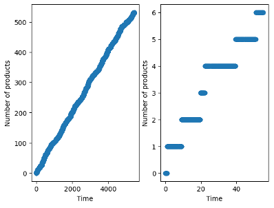
Figure 2: Number of products formed as a function of simulation time after a long time (left) and shorter time interval (right).

Steady-state B formation rates and surface coverages are obtained by taking time-averages of these quantities over a long enough simulation time. Rates are obtained by normalizing the number of products formed by the time elapsed:

#calculate rates

rates = np.sum(N_Ps)/np.sum(ts)

Coverages are obtained by finding the amount of time the system exists in each state, and normalizing by the total simulation time, shown for a vacant surface, for instance, with L=0:

#convert Ls into np array, and get rid of last element to report time elapsed for coverages

Ls_np = np.array(Ls[0:-1])

#indexes where surface is vacant (L==0)

L0_ind = np.where(Ls_np == 0)

ts_np = np.array(ts)

#time elapsed in for each instance where L==0

time_L0 = np.sum(ts_np[L0_ind[0]+1]-ts_np[L0_ind[0]])

#normalize vacant time with total elapsed time

cov_v = time_L0/ts_np[-1]

The simulation coverages and rates can be reported from these averages as follows:

* coverage: 0.09190093419008047

A coverage: 0.9072329666594803

B coverage: 0.09190093419008047

rates: 0.0891111360522377

Comparing kMC simulation results to the mean-field kinetic description:

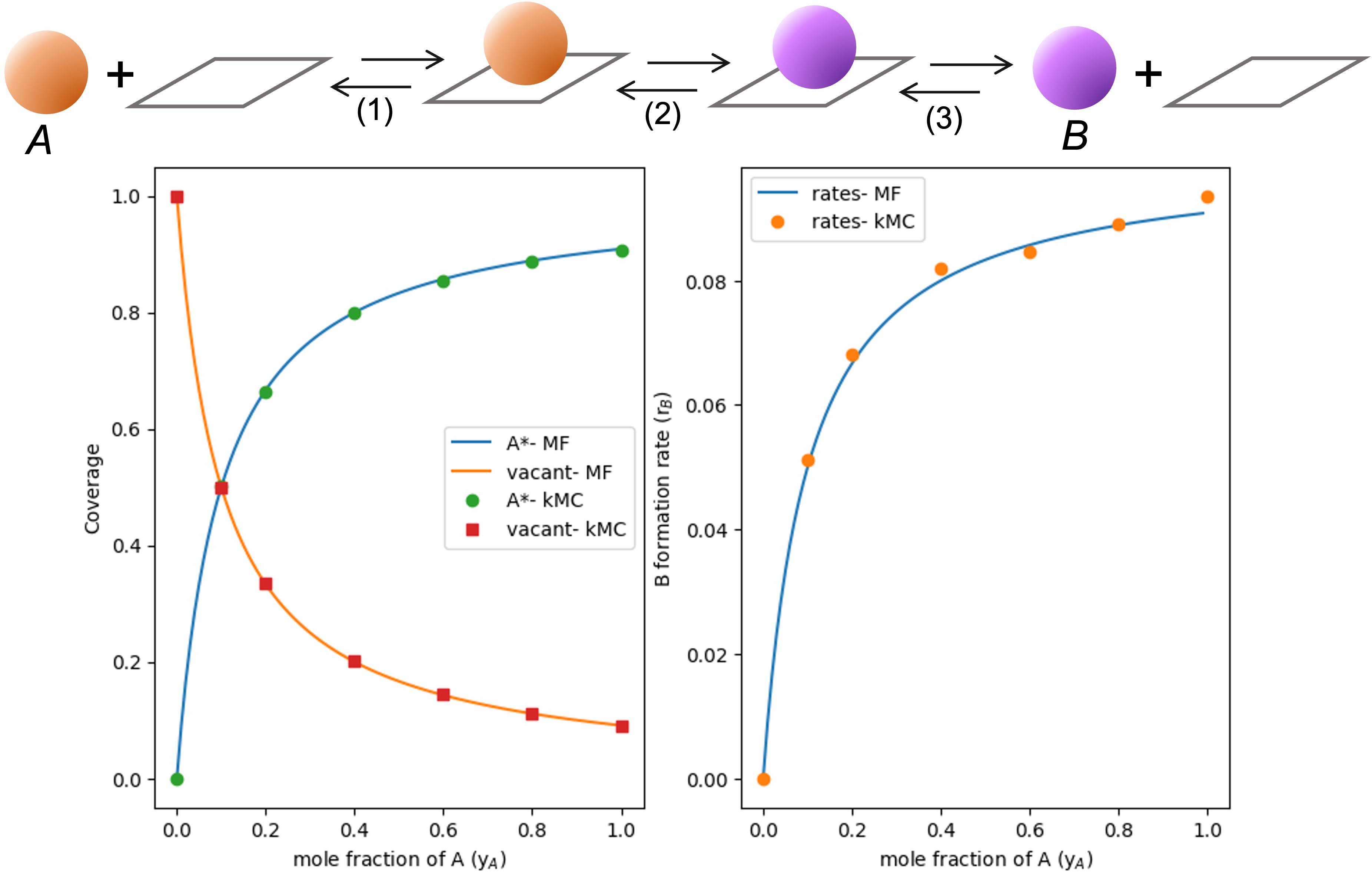
The rate of B formation for a y_A value of unity was found to be 0.089 from the kMC simulation, which is similar to the pseudo-steady state value obtained from the mean-field equation in equation 8 (0.091). The trends for coverage and rates with changing y_A values, but constant (zero) y_B values, are obtained by initializing the simulation with different numbers of N_A, for a fixed total number of species in the reservoir, denoted as N_tot:

# initialize:

…

N_tot = 1000

Then, kA_a and kB_a values are parameterized based on N_A and N_B normalized by N_tot, instead of by the sum of N_A and N_B, to reflect other inert species (like He) making up the balance in the reservoir:

for i in range(trials):

…

if L == 0: #vacant site

kA_a = kA_a0 * (N_A)/(N_tot)

kB_a = kB_a0 * (N_B)/(N_tot)

Running the simulation for a series of N_A values, and constant N_tot and N_B (zero), reproduces the trend from Figure 1. These data are shown alongside the results from the mean field kinetic model in Figure 3. The close agreement between mean-field descriptions and kMC simulations shows how time-averaged behaviours from a reactions on single site with discrete descriptions of site occupancy and product formation report the same kinetic trends as continuous mean field descriptions. Such agreement reflects the fact that the kMC simulation samples the same distribution of states as the ensemble considered in deriving the Langmuir-Hinshellwood kinetic expressions.

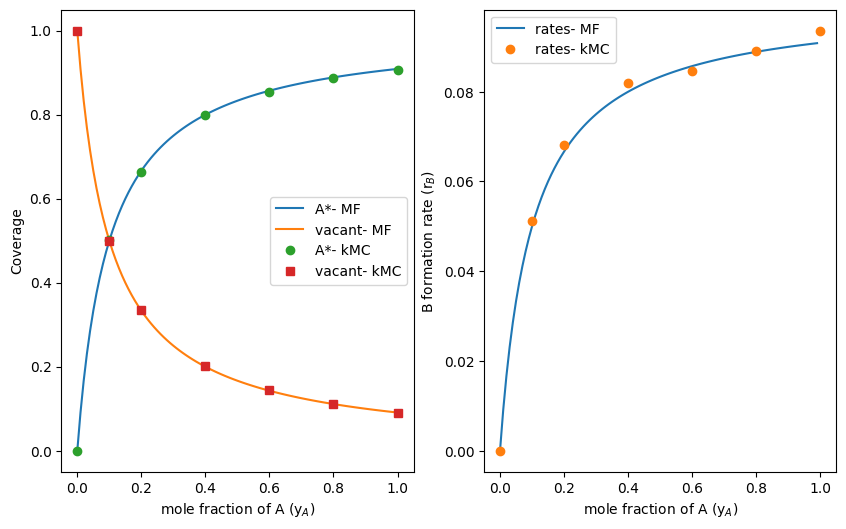
Figure 3: Coverage of A* and vacant *-sites (Left) and B formation rates as a function of y_A mole fractions from mean-field descriptions (MF) and time-averaged behaviours from kMC simulations (kMC).

Exercises:

1. Compare rates obtained from different simulation times to see how much the average values vary, and how long a sampling time is necessary to obtain reliable reported values.

2. What changes to the rate constants in Table 1 invalidate the assumptions made in deriving equation 8? How can this be probed with the kMC simulation?

3. Adapt the code to consider a more complex reaction like A<->A*<->B*<->C*

References:

[1] Andersen M, Panosetti C, Reuter K. A Practical Guide to Surface Kinetic Monte Carlo Simulations. Front Chem. 2019;7:202.

[2] Reaction rate theory and rare events (Chapter 14). B Peters. Elsevier, 2017. ISBN: 978-0-444-56349-1

Appendix:

The sample code is available as a Jupyter notebook entitled “kMC_A_B_rxn_single_site_eq.ipynb” at the ari-fischer GitHub page (https://github.com/ari-fischer/) in the “kinetics_tutorial” repository under the “KMC_tutorials” folder